Time Series Data with InfluxDB and Grafana

Last updated: 2023-11-24

On the face of it, the collection of metrics can appear deceptively simple - after all, they consist of simple types such as labels, numbers and timestamps. When modern distributed systems generate tens of billions of records per day though, the picture becomes much more complex. That data needs to be ingested, stored and analysed at high speed. This can result in huge storage costs as well as requiring massive computational power. To meet these challenges, a number of dedicated time series databases have appeared on the market in recent years. One of the most popular of these is InfluxDB. InfluxDB is something of a veteran - having been around in one form or another for over 10 years - and now boasts over 500,000 active users. It promises high performance and scalability at a competitive price.

InfluxDB is open source and is available in both cloud and self-hosted versions. In this article we will look at

setting up a simple InfluxBb instance
formatting and ingesting a metrics file
visualizing the data in Grafana

All of the steps can be followed using the free versions of both tools.

InfluxDB Cloud Serverless

We are going to be using the InfluxDb Cloud Serverless tier. This tier provides us with an allocation of two "buckets" - which are synonymous to databases. In addition to this limitation, the buckets only have a maximum retention period of 30 days. As this is a time series database the term 'retention period' has a specialised meaning. It does not simply mean that any row of data submitted to the API will be retained for thirty days. It actually means that the timestamp field of the row cannot be more than 30 days in the past. Setting up a cloud account is an extremely simple process. As you can see below, the sign-up screen only requires a few basic details:

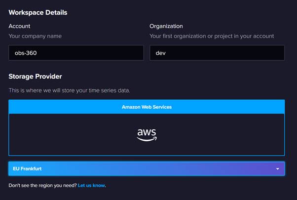
Once we have created our account, we just need to enter some workspace details:

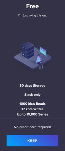
And then confirm that we want to use the free plan:

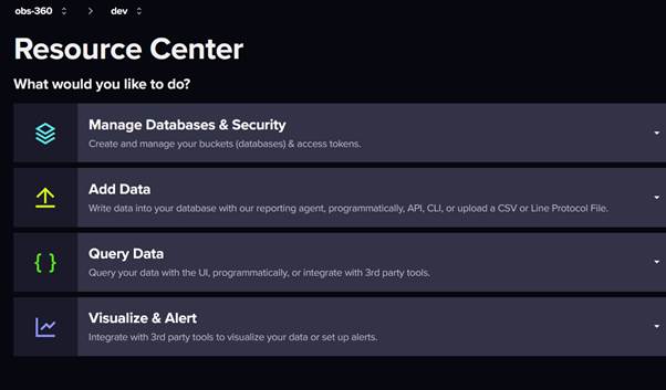
Now we are ready to add our data.

Adding Data

Our aim is to upload some time series data to InfluxDB and then visualize that data in Grafana. There are numerous methods for uploading data to InfluxDB:

The InfluxDb API
The CLI
Uploading a file via the UI

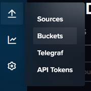
We are going to attempt to upload a CSV containing a set of weather data using the InfluxDB CLI. As we said earlier - InfluxDB has the concept of a 'bucket' - which is roughly synonymous to a database. So we are going to create a bucket and then try to upload our data to that bucket. We will select the Buckets option from the side menu:

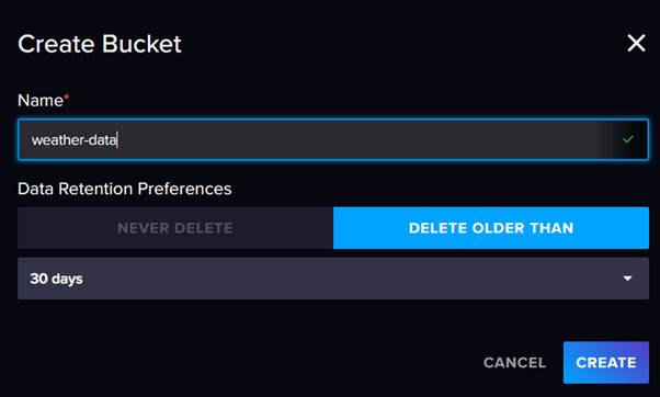
And then click on the Create Bucket button:

We are going to call our bucket 'weather-data' and accept the default retention period of 30 days (which is the maximum we are allowed in the free plan).

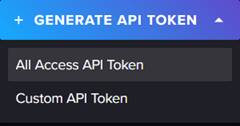
Now that our bucket is created, we can start to think about populating it with data. As we are going to use the CLI we will obviously need to install the CLI tool. The CLI can be downloaded from this url on the InfluxDB web site. Installation is just a simple matter of downloading the zipped executable and then unzipping it and copying it to a folder. Next, we need to generate a token that the CLI can use when communicating with the InfluxDB API. When you click on the API Tokens menu option you will have the option to create either an 'All Access API Token' or a 'Custom API Token'. The principle of least privilege dictates that we should create a custom token:

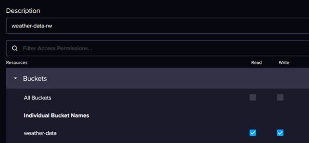
We are going to assign the token read and write permissions on our weather data bucket:

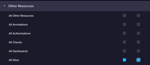
We will also assign a 'dbrp' (database retention policy) permission, which we will need later on:

As well as an Org permission:

User Configuration

The next thing we are going to do is create an InfluxDB user configuration. This is a set of attributes that the CLI uses when authenticating itself to the InfluxDB API. Saving the details in a configuration saves us having to pass them in every time we make a call to the API: The syntax for creating the configuration is:

    
   .\influx config create  --config-name  \
    --host-url  \
    --org  \
    --token

To connect to a cloud instance you enter the fully qualified domain part of the InfluxDb url that you see in your browser. In my case it is: 'https://eu-central-1-1.aws.cloud2.influxdata.com'
You do not need to enter anything after the '.com' segment. The command we will run will therefore look something like this:

    
    .\influx config create�� --config-name weather-config� --host-url� https://eu-central-1-1.aws.cloud2.influxdata.com�� --org dev�� --token 1234

If the command runs successfully, you will see a confirmation like this:

Data Structure and Annotations

Now it is time for us to get some data into our bucket. In a real-world situation you would probably have a service which was continually streaming data into the InfluxDB API. To keep things simple, we are just going to upload data from a CSV file. Our file is called weather-data-us.csv and it contains 996 records. These are fictitious readings of weather metrics for a single day taken at one minute intervals. You can find this file in our GitHub repo . If you do use this file, you may need to update the values for the time field to ensure that they fall within the last 30 days, otherwise the InfluxDB API will be reject them as being outside of the retention period. 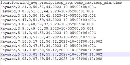The structure of the CSV is shown below:

As you can see, we have a location field followed by values for wind, rain and temperature and then a timestamp field. We are going to use the CLI's 'write' command to upload our data. This just requires us to pass in the name of our file and the name of the bucket we want to write to. Ok, lets go ahead and run our command

                    
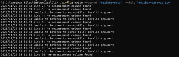
  .\influx write --bucket "weather-data"� --file "weather-data-us.csv"

Ooops - kaboom!

Even though we have uploaded a correctly formatted csv file, it is not yet valid for ingestion into InfluxDB. The reason for this is that before InfluxDB can ingest our data, it first of all needs to understand its shape - otherwise it will not be able to store and retrieve the data optimally. We need to provide 'annotations' which describe the data and tell InfluxDB how to process it. In particular, we need to provide a 'measurement' and describe the types of data we are passing. 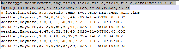You can find out more about annotations in the InfluxDB Cloud Serverless Documentation We are now going to update our csv file with the required annotations:

You will see that we have inserted two lines at the top of the file. The first row defines the structure of the data. You will see the first value after the '#datatype' declaration is the word 'measurement'. Every file we submit must define a measurement. This is kind of akin to assigning a table name for our data so that InfluxDB can group our data together logically. We have also inserted a new column with the name of our measurement - i.e. 'weather'. Although this seems a little bit redundant, it makes sense when you realise that we can supply multiple measurements/tables in the same file and InfluxDB needs some way of distinguishing between them. The revised file is named "weather-data-us-2.csv" and is also in the GitHub repo. We will run our command again - this time pointing to the new file:

                    
.\influx write --bucket "weather-data"� --file "weather-data-us-2.csv"

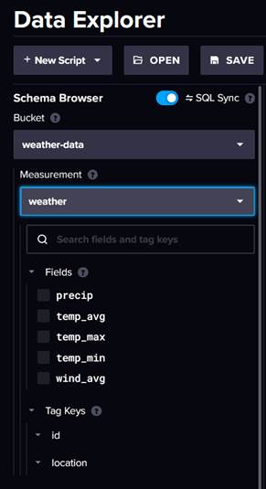
If the Write command succeeds, the CLI does not actually send any response to your terminal. We can, however, verify that the write was successful by checking in the InfluxDB UI. In the Data Explorer we can select our bucket (weather-data) and our measurement (weather), and we will then see a list of fields:

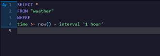
You will also see that the Data Explorer auto-generates a query for us so that we can view our data:

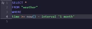
This query defaults to looking at records for the past hour. Our data is not this fresh so we will change the query to bring back data from the past month:

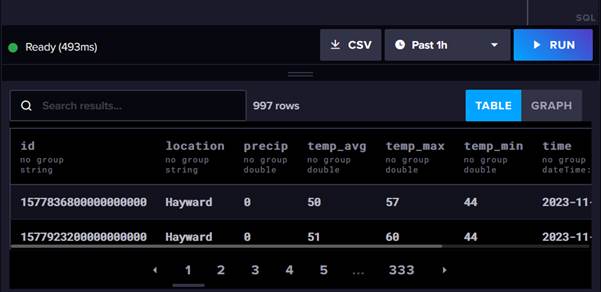
When we run the query, we will see that 996 records are returned:

dbrp Mapping

We can now view our data in the InfluxDB UI. However, we have one more configuration step to complete to make our bucket accessible to Grafana. InfluxDB supports different languages for querying our data - including Flux and InfluxQL. Flux is a powerful querying tool, but we are going to use InfluxQL as its syntax is close to the SQL syntax that many of us are familiar with. There is a slight complication when we do this though. There seems to be a bit of a mis-alignment between the current Grafana connectors and different versions of InfluxDB backend API's. In Version 1 of InfluxDB, the backend store was a database and the query language was InfluxQL. With version two, databases were replaced with buckets and Flux became the primary query language. Grafana therefore seems to assume that, if you wish to use InfluxQL as your query language, you are talking to an InfluxDB 1 database rather than an InfluxDB 2 bucket. Appendix 1 below provides some more detail on this.

To get around this discrepancy we need to create a mapping. The mapping takes the name of a database and the name of a retention policy and then maps these to our Bucket. Neither the database nor the retention policy that you define actually need to exist! They are just placeholders to enable us to create a mapping. This does sound a little bit counter-intuitive - on the upside though, the command for creating the mapping is pretty simple. From the InfluxDB command line we just need to run the v1 dbrp create command. This command takes three parameters:

bucket-id - this is the alphanumeric id, not the name of our bucket
db - a placeholder database name
rp - a placeholder retention policy name

Our command will look like this:

    
    .\influx v1 dbrp create�� --bucket-id 12345678�� --db� weatherdb� --rp weather-db-rp -c weather-config

If the command executes successfully, you will see an response like this:

Visualizing InfluxDB Metrics in Grafana

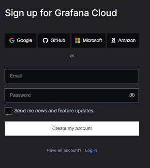
Having successfully imported our data into InfluxDB, we move on to the second part of the exercise - visualizing the data in Grafana. As we said earlier, we are going to be using the Grafana Cloud free tier. As with InfluxDB, signing up is as easy as falling off a log. Simply head over to the sign-up page.

As you can see, you can either provide an email and password or use one of the selected identity providers. Once our account has been created, we just need to create a Data Source and then create a visualization which uses that data source.

Creating a Data Source

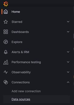
On your home page just click on the hamburger icon in the top left of the page:

And then click on Data Sources:

Next, click on the Add New Data Source button and then select the InfluxDB option:

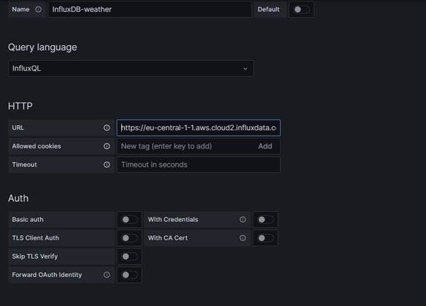
We will now:

Enter a name for the data source
Select InfluxQL as the query language for our data source
Enter the Url of our InfluxDB endpoint

Next, we need to add a Custom HTTP header for authorization. Populate the values for the header as follows:

Header:Authorization
Value: Token <your API token> (don't include the angle brackets!).

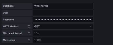
Finally, we add the database connection details:

The Database will be the name we specified when we created our dbrp mapping
The User field is left blank
The Password is our API token.

Next click on Save and Test and you should see a confirmation that our data source is working:

Our configuration is now complete and we can move on to creating our visualization.

Creating a Visualization

From the Grafana home page click on Dashboards, then New/New Dashboard. Then click on the big blue Add Visualization button:

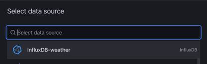
You will then be prompted to select a Data Source, so obviously we will select the InfluxDB-weather data source we created earlier.

Once the Data Source has been selected, the Edit Panel page will load. The first thing you will see is a notice in the middle of the panel telling us that, unfortunately, there is no data to display.

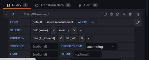
This is not surprising as, even though we have specified a data source, we have not defined a query for retrieving the data. In the same way that a relational database has many tables, an InfluxDB Bucket can have many measurements. We need to supply an InfluxQL query specifying which measurement and which fields we want to retrieve. If we look at the lower section of our screen, we can see that we can use a query builder to create our query.

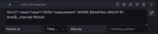
Instead of this, we are going to click on the pencil icon and enter raw InfluxQL:

Initially, the query editor will display a query which is syntactically valid but which is non-functional for us. We can see, however, that we need to specify a measurement and also select one or more� fields to display. We have called our measurement �weather�. In our query, we also have to qualify this with the name of the database retention policy it maps to, as shown below:

We also need to update the date range for the query. This defaults to the past six hours but we are going to specify an exact data range to match the data in our file:

If you now hit the dashboard refresh button

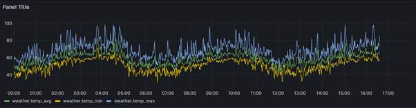
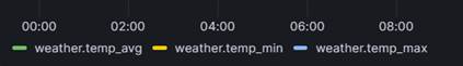
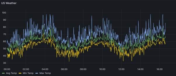
You should see a gorgeous line graph:

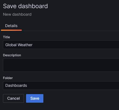
Next we just need to give our panel a title - we are going to call it �US Weather�. Then we will save our dashboard:

Overrides

Our dashboard looks great, but there is one niggle - the labels on the legend are rather unsightly.

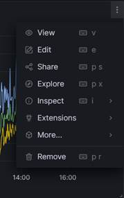
It would be better to have more readable wording rather than just displaying the field names from our bucket. To tidy this up we are going to use a very powerful Grafana feature called 'Overrides'. Overrides allow us to re-format the way that data is presented without having any side-effects on the shape of the underlying data stream itself. If you hover over the top right of the panel, you will see three dots and clicking on those will bring up a context menu.

Click on Edit and when the Edit Panel screen appears scroll down the Panel Options column on the right-hand side of the screen. Now click on the 'Add field override' button.

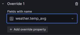
Next select the 'Fields with name' option and select the �weather.temp_avg� field. Next click on the 'Add override property' button:

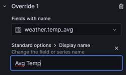
This will bring up a long list of properties that you can override. Scroll through the list and select 'Standard options > Display name'. We will now have a text box where we can enter a prettier name for our label.

As soon as you press the Enter key the legend will be updated with the new label value. We now just need to repeat the process for our other two fields and then save our changes:

Ok - that looks perfect! We can wrap things up.

Summary

In this exercise we have seen how we can use free offerings from InfluxDB and Grafana to ingest and visualize time series data. Although getting set up with InfluxDB is a breeze, it can't simply be used as a data dump. The nature of time series databases means that we need to sculpt our data and provide annotations. We have also seen how easy it is to use the InfluxDB CLI to push data into its API once we have prepared it correctly. We have also seen that the built-in InfluxDB connector in Grafana makes it simple to connect to an InfluxDB data source. We have constructed a simple InfluxQL query and even used an Override to transform our data labels.

In some ways we have covered quite a bit of ground here. In others, we have hardly scratched the surface. These are industrial strength products capable of handling throughputs on a massive scale and generating visualisations of enormous complexity. However, being able to ingest data to a tool like InfluxDB and then connect to it in Grafana gives us a great foundation for further exploration.

Appendix 1

At the moment some of the messages around Flux can be a little disorienting when using the InfluxDB/Grafana stack. In Grafana you will see warnings that their support for Flux is in Beta. This might give the impression that Flux is hot off the InfluxDB press.

In InfluxDB though, you will see warnings that Flux is going into maintenance mode:

The full text of the above notification is as follows:

The future of Flux
Flux is going into maintenance mode. You can continue using it as you currently are without any changes to your code.

Flux is going into maintenance mode and will not be supported in InfluxDB 3.0. This was a decision based on the broad demand for SQL and the continued growth and adoption of InfluxQL. We are continuing to support Flux for users in 1.x and 2.x so you can continue using it with no changes to your code. If you are interested in transitioning to InfluxDB 3.0 and want to future-proof your code, we suggest using InfluxQL.

For information about the future of Flux, see the following:
The plan for InfluxDB 3.0 Open Source
InfluxDB 3.0 benchmarks

Jay Clifford - who is a Developer Advocate for InfluxDB, goes into more detail on the ins and outs of InfluxQL in this blog post.

If you have any comments or feedback on this article, please get in touch: